Gradient Descent for Linear Regression

Today I am going to use Octave to perform Gradient Descent for Linear Regression.

Reminder of how to plot charts with Octave

Before I begin, below are a few reminders on how to plot charts using Octave.

Given we have data in a csv with 2 columns for data X and Y. We can plot charts using Octaves plot function. For convenience I have wrapped this in a "plotData" function which also adds in the X and Y Labels to the axes. This function has also set our market size to "15".

The data is then pulled in using the load function and fed to our plotData function providing the beutiful chart below.

Plotting graphs function

function plotData(x, y)

figure; % open a new figure window

plot(x,y,'rx','MarkerSize',15);
ylabel('Y');
xlabel('X');

print -dsvg data.svg % prints figure to an svg file

end

Example code generating the plot

fprintf('Plotting Data ...\n')
data = load('data.csv');
X = data(:, 1); y = data(:, 2);

plotData(X, y);

Scatter Plot

Linear Regresssion with Gradient Descent

Gradient Descent is an algorithm for minimizing a function. We can apply this to Linear regression by constructiong a cost function for Linear regression

Code to create grid of CostFunction Values for Theta

fprintf('Visualizing J(theta_0, theta_1) ...\n')

% Grid over which we will calculate J
theta0_vals = linspace(-10, 10, 100);
theta1_vals = linspace(-1, 4, 100);

% initialize J_vals to a matrix of 0's
J_vals = zeros(length(theta0_vals), length(theta1_vals));

% Fill out J_vals
for i = 1:length(theta0_vals)
    for j = 1:length(theta1_vals)
      t = [theta0_vals(i); theta1_vals(j)];
      J_vals(i,j) = computeCost(X, y, t);
    end
end

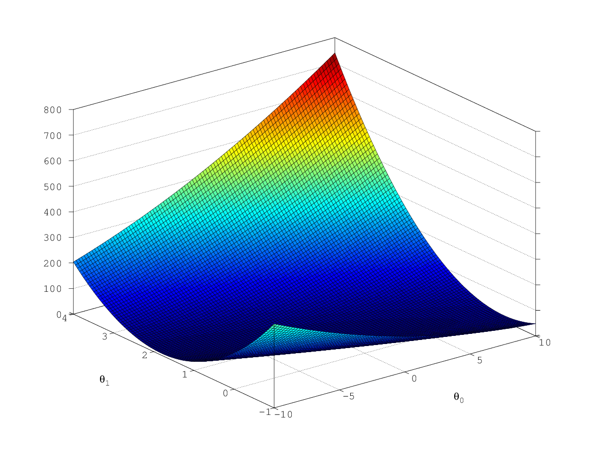
J_vals = J_vals';

To get an idea of the function we are trying to minimise, I have plotted the cost function values below. Using Gradient Descent we want to work towards

finding the global minimum of the cost function which would be the lowest most point in the graph Below.

This lowest point corresponds to the linear regression parameters with the smallest error.

Code to plot a surface diagram using grid of costFunction Values above

% Surface plot
figure;

surf(theta0_vals, theta1_vals, J_vals);
xlabel('\theta_0'); ylabel('\theta_1');
print -dpng datasurf.png;
fprintf('finished surf diagram\n')

Surface Plot of Cost Function

Another way to view this same cost function is using a contor plot.

Code to create contour plot

figure;
% Plot J_vals as 15 contours spaced logarithmically between 0.01 and 100
contour(theta0_vals, theta1_vals, J_vals, logspace(-2, 3, 20))
xlabel('\theta_0'); ylabel('\theta_1');
hold on;

plot(theta(1), theta(2), 'rx', 'MarkerSize', 10, 'LineWidth', 2);
hold off;
print -dsvg datacontour.svg;

Contour Plot of Cost Function

Performing Gradient Descent

When we performing gradient descent for Linear regression we are trying to minimize the following equation

find min of $$J (\theta)$$ where $$J(\theta) =\frac{1}{2m} \sum_{i=1}^m \epsilon_i^2 = \frac{1}{2m} \sum_{i=1}^m (h_\theta (x^{(i)}) - y^{(i)})^2$$ and $$h_\theta (x) = \theta^Tx$$

and

• $m$ is the number of training examples for our algorithm
• $x$ is our features or input data
• $y$ is our output

In the case where x has only one feature: $$\theta^Tx = \theta_0 + \theta_1x_1$$

Instead of calculating this directly by using the the standard linear regression we will be using gradient descent.

More about Linear regression in general can be found here: * Wikipedia:Simple linear regression

Running Gradient descent with Octave

To perform gradient descent we will try to minimize the cost function $J(\theta)$ incrementally.

To do this we will repeatedly apply the following update to $\theta$

$$\theta_j := \theta_j - \alpha \frac{1}{m}\sum_{i=1}^m (h_\theta(x^{(i)}) - y^{(i)})x_j^{(i)}$$

It turns out that the above equation is the derivative of the cost function with respect to theta and this can direct us to the optimal and minimal value of the cost function. (given appropriate $\alpha$)

function J = computeCost(X, y, theta)
m = length(y); % number of training examples
J =  1/(2*m) *  sum( ( X*theta - y) .^ 2);
end

function [theta, J_history] = gradientDescent(X, y, theta, alpha, num_iters)

m = length(y); % number of training examples
J_history = zeros(num_iters, 1);

for iter = 1:num_iters


    AB1 = X * theta;
    AB2 = AB1 - y;
    AB3 = AB2' * X;
    theta = theta - alpha * (1/m) * AB3';
    J_history(iter) = computeCost(X, y, theta);
end

Note that we also return the cost function. If we see that this converges we know that the gradient descent is converging to a minimal value.

Credit

I learned most of the above by following Andrew Ng's course on machine learning, which I would highly recommend taking.

• Coursera - Machine Learning by Andrew Ng at Stanford University